Category: Code
Brief GDB Basics
In this post I would like to go through some of the very basic cases in which gdb can come in handy. I’ve seen people avoid using gdb, saying it is a CLI tool and therefore it would be hard to use. Instead, they opted for this:
std::cout << "qwewtrer" << std::endl;
DEBUG("stupid segfault already?");
That’s just stupid. In fact, printing a back trace in gdb is as easy as writing two letters. I don’t appreciate lengthy debugging sessions that much either, but it’s something you simply cannot avoid in software development. What you can do to speed things up is to know the right tools and to be able to use them efficiently. One of them is GNU debugger.
Example program
All the examples in the text will be referring to the following short piece of code. I have it stored as segfault.c and it’s basically a program that calls a function which results in segmentation fault. The code looks like this:
/* Just a segfault within a function. */

#include <stdio.h>
#include <unistd.h>

void segfault(void)
{
	int *null = NULL;
	*null = 0;
}

int main(void)
{
	printf("PID: %d\n", getpid());
	fflush(stdout);

	segfault();

	return 0;
}
Debugging symbols
One more thing, before we proceed to gdb itself. Well, two actually. In order to get anything more than a bunch of hex addresses you need to compile your binary without stripping symbols and with debug info included. Let me explain.
Symbols (in this case) can be thought of simply variable and function names. You can strip them from your binary either during compilation/linking (by passing -s argument to gcc) or later with strip(1) utility from binutils. People do this, because it can significantly reduce size of the resulting object file. Let’s see how it works exactly. First, compile the code with striping the symbols:
[astro@desktop ~/MyBook/code]$ gcc -s segfault.c
Now let’s fire up gdb:
[astro@desktop ~/MyBook/code]$ gdb ./a.out
GNU gdb (GDB) Fedora (7.3.1-48.fc15)
Reading symbols from /mnt/MyBook/code/a.out...(no debugging symbols found)...done.
Notice the last line of the output. gdb is complaining that it didn’t find any debuging symbols. Now, let’s try to run the program and display stack trace after it crashes:
(gdb) run
Starting program: /mnt/MyBook/code/a.out
PID: 21568

Program received signal SIGSEGV, Segmentation fault.
0x08048454 in ?? ()
(gdb) bt
#0  0x08048454 in ?? ()
#1  0x0804848d in ?? ()
#2  0x4ee4a3f3 in __libc_start_main (main=0x804845c, argc=1, ubp_av=0xbffff1a4, init=0x80484a0, fini=0x8048510,
    rtld_fini=0x4ee1dfc0 , stack_end=0xbffff19c) at libc-start.c:226
#3  0x080483b1 in ?? ()
You can imagine, that this won’t help you very much with the debugging. Now let’s see what happens when the code is compiled with symbols, but without the debuginfo.
[astro@desktop ~/MyBook/code]$ gcc segfault.c
[astro@desktop ~/MyBook/code]$ gdb ./a.out
GNU gdb (GDB) Fedora (7.3.1-48.fc15)
Reading symbols from /mnt/MyBook/code/a.out...(no debugging symbols found)...done.
(gdb) run
Starting program: /mnt/MyBook/code/a.out
PID: 21765

Program received signal SIGSEGV, Segmentation fault.
0x08048454 in segfault ()
(gdb) bt
#0  0x08048454 in segfault ()
#1  0x0804848d in main ()
As you can see, gdb still complains about the symbols in the beginning, but the results are much better. The program crashed when it was executing segfault() function, so we can start looking for any problems from there. Now let’s see what we get when debuginfo get’s compiled in.
[astro@desktop ~/MyBook/code]$ gcc -g segfault.c
[astro@desktop ~/MyBook/code]$ gdb ./a.out
GNU gdb (GDB) Fedora (7.3.1-48.fc15)
Reading symbols from /mnt/MyBook/code/a.out...done.
(gdb) run
Starting program: /mnt/MyBook/code/a.out
PID: 21934

Program received signal SIGSEGV, Segmentation fault.
0x08048454 in segfault () at segfault.c:9
9		*null = 0;
That’s more like it! gdb printed the exact line from the code that caused the program to crash! That means, every time you try to use gdb to get some useful directions for debugging, make sure, that you don’t strip symbols and have debuginfo available!
Start, Stop, Interrupt, Continue
These are the basic commands to control your application’s runtime. You can start a program by writing
(gdb) run
When a program is running, you can interrupt it with the usual Ctrl-C, which will send SIGINTR to the debugged process. When the process is interrupted, you can examine it (this is described later in the post) and then either stop it completely or let it continue. To stop the execution, write
(gdb) kill
If you’d like to let your program carry on executing, use
(gdb) continue
I should point out, that in gdb, you can abbreviate most of the commands to as little as a single character. For instance r can be used for run, k for kill, c for continue and so on :).
Stack traces
Stack traces are very powerful when you need to localize the point of failure. Seeing a stack trace will point you directly to the function, that caused you program to crash. If your project is small or you keep your functions short and straight-forward, this could be all you’ll ever need from a debugger. You can display stack trace in case of a segmentation fault or generally anytime when the program is interrupted. The stack trace can be displayed by a backtrace or bt command
(gdb) bt
#0  0x08048454 in segfault () at segfault.c:9
#1  0x0804848d in main () at segfault.c:17
You see, that the program stopped (more precisely was killed by the kernel with a SIGSEGV signal) at line 9 of segfault.c file while it was executing a function segfault(). The segfault function was called directly from the main() function.
Listing source code
When the program is interrupted (and compiled it with debuginfo), you can list the code directly by using the list command. It will show the precise line of code (with some context) where the program was interrupted. This can be more convenient, because you don’t have to go back into your editor and search for the place of the crash by line numbers.
(gdb) list
4 #include
5
6 void segfault(void)
7 {
8   int *null = NULL;
9 *null = 0;
10 }
11
12 int main(void)
13 {
We know (from the stack trace), that the program has stopped at line 9. This command will show you exactly what is going on around there.
Breakpoints
Up to this point, we only interrupted the program by sending a SIGTERM to it manually. This is not very useful in practice though. In most cases, you will want the program stop at some exact place during the execution, to be able to inspect what is going on, what values do the variables have and possibly to manually step further through the program. To achieve this, you can use breakpoints. By attaching a breakpoint to a line of code, you say that you want the debugger to interrupt every time the program wants to execute the particular line and wait for your instructions.
A breakpoint can be set by a break command (before the program is executed) like this
(gdb) break 8
Breakpoint 2 at 0x4005c0: file segfault.c, line 8.
I’m using line number to specify, where to put the break, but you can use also function name and file name. There are multiple variants of arguments to break command.
You can list the breakpoints you have set up by writing info breakpoints:
(gdb) info breakpoints
Num     Type           Disp Enb Address            What
1       breakpoint     keep n   0x00000000004005d8 in main at segfault.c:14
2       breakpoint     keep y   0x00000000004005c0 in segfault at segfault.c:8
To disable a break point, use disable <Num> command with the number you find in the info.
Stepping through the code
When gdb stops your application, you can resume the execution manually step-by-step through the instructions. There are several commands to help you with that. You can use the step and next commands to advance to the following line of code. However, these two commands are not entirely the same. Next will ‘jump’ over function calls and run them at once. Step, on the other hand, will allow you to descend into the function and execute it line-by-line as well. When you decide you’ve had enough of stepping, use the continue command to resume the execution uninterrupted to the next break point.
Breakpoint 1, segfault () at segfault.c:8
8		int *null = NULL;
(gdb) step
9		*null = 0;
There are multiple things you can do during the process of stepping through a running program. You can dump values of variables using the print command, even set values to variables (using set command). And this is definitely not all. Gdb is great! It really can save a lot of time and lets you focus on the important parts of software development. Think of it the next time you try to bisect errors in the program by inappropriate debug messages :-).
Sources
Magical container_of() Macro
When you begin with the kernel, and you start to look around and read the code, you will eventually come across this magical preprocessor construct. What does it do? Well, precisely what its name indicates. It takes three arguments — a pointer, type of the container, and the name of the member the pointer refers to. The macro will then expand to a new address pointing to the container which accommodates the respective member. It is indeed a particularly clever macro, but how the hell can this possibly work? Let me illustrate …
The first diagram illustrates the principle of the container_of(ptr, type, member) macro for who might find the above description too clumsy.

Illustration of how containter_of macro works
Bellow is the actual implementation of the macro from Linux Kernel:
#define container_of(ptr, type, member) ({                      \
        const typeof( ((type *)0)->member ) *__mptr = (ptr);    \
        (type *)( (char *)__mptr - offsetof(type,member) );})
At first glance, this might look like a whole lot of magic, but it isn’t quite so. Let’s take it step by step.
Statements in Expressions
The first thing to gain your attention might be the structure of the whole expression. The statement should return a pointer, right? But there is just some kind of weird ({}) block with two statements in it. This in fact is a GNU extension to C language called braced-group within expression. The compiler will evaluate the whole block and use the value of the last statement contained in the block. Take for instance the following code. It will print 5.
int x = ({1; 2;}) + 3;
printf("%d\n", x);
typeof()
This is a non-standard GNU C extension. It takes one argument and returns its type. Its exact semantics is throughly described in gcc documentation.
int x = 5;
typeof(x) y = 6;
printf("%d %d\n", x, y);
Zero Pointer Dereference
But what about the zero pointer dereference? Well, it’s a little pointer magic to get the type of the member. It won’t crash, because the expression itself will never be evaluated. All the compiler cares for is its type. The same situation occurs in case we ask back for the address. The compiler again doesn’t care for the value, it will simply add the offset of the member to the address of the structure, in this particular case 0, and return the new address.
struct s {
	char m1;
	char m2;
};

/* This will print 1 */
printf("%d\n", &((struct s*)0)->m2);
Also note that the following two definitions are equivalent:
typeof(((struct s *)0)->m2) c;

char c;
offsetof(st, m)
This macro will return a byte offset of a member to the beginning of the structure. It is even part of the standard library (available in stddef.h). Not in the kernel space though, as the standard C library is not present there. It is a little bit of the same 0 pointer dereference magic as we saw earlier and to avoid that modern compilers usually offer a built-in function, that implements that. Here is the messy version (from the kernel):
#define offsetof(TYPE, MEMBER) ((size_t) &((TYPE *)0)->MEMBER)
It returns an address of a member called MEMBER of a structure of type TYPE that is stored in memory from address 0 (which happens to be the offset we’re looking for).
Putting It All Together
#define container_of(ptr, type, member) ({                      \
        const typeof( ((type *)0)->member ) *__mptr = (ptr);    \
        (type *)( (char *)__mptr - offsetof(type,member) );})
When you look more closely at the original definition from the beginning of this post, you will start wondering if the first line is really good for anything. You will be right. The first line is not intrinsically important for the result of the macro, but it is there for type checking purposes. And what the second line really does? It subtracts the offset of the structure’s member from its address yielding the address of the container structure. That’s it!
After you strip all the magical operators, constructs and tricks, it is that simple :-).
References
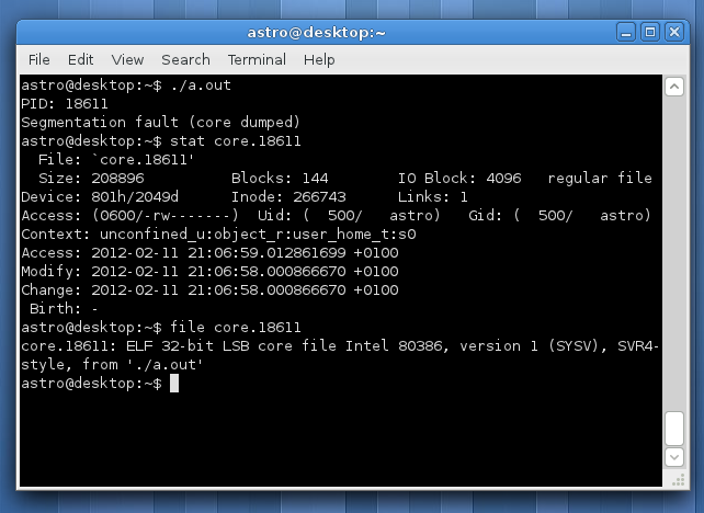
Core dumps in Fedora
This post will demonstrate a way of obtaining and examining a core dump on Fedora Linux. Core file is a snapshot of working memory of some process. Normally there’s not much use for such a thing, but when it comes to debugging software it’s more than useful. Especially for those hard-to-reproduce random bugs. When your program crashes in such a way, it might be your only source of information, since the problem doesn’t need to come up in the next million executions of your application.
The thing is, creation of core dumps is disabled by default in Fedora, which is fine since the user doesn’t want to have some magic file spawned in his home folder every time an app goes down. But we’re here to fix stuff, so how do you turn it on? Well, there’s couple of thing that might prevent the cores to appear.
1. Permissions
First, make sure that the program has writing permission for the directory it resides in. The core files are created in the directory of the executable. From my experience, core dump creation doesn’t work on programs executed from NTFS drives mounted through ntfs3g.
2. ulimit
This is the place where the core dump creation is disabled. You can see for yourself by using the ulimit command in bash:
astro@desktop:~$ ulimit -a
core file size          (blocks, -c) 0
data seg size           (kbytes, -d) unlimited
scheduling priority             (-e) 0
file size               (blocks, -f) unlimited
pending signals                 (-i) 15976
max locked memory       (kbytes, -l) 64
max memory size         (kbytes, -m) unlimited
open files                      (-n) 1024
pipe size            (512 bytes, -p) 8
POSIX message queues     (bytes, -q) 819200
real-time priority              (-r) 0
stack size              (kbytes, -s) 8192
cpu time               (seconds, -t) unlimited
max user processes              (-u) 1024
virtual memory          (kbytes, -v) unlimited
file locks                      (-x) unlimited
To enable core dumps set some reasonable size for core files. I usually opt for unlimited, since disk space is not an issue for me:
ulimit -c unlimited
This setting is local only for the current shell though. To keep this settings, you need to put the above line into your ~/.bashrc or (which is cleaner) adjust the limits in /etc/security/limits.conf.
3. Ruling out ABRT
In Fedora, cores are sent to the Automatic Bug Reporting Tool — ABRT. So they can be posted to the RedHat bugzilla to the developers to analyse. The kernel is configured so that all core dumps are pipelined right to abrt. This is set in /proc/sys/kernel/core_pattern. My settings look like this
|/usr/libexec/abrt-hook-ccpp %s %c %p %u %g %t %h %e 636f726500
That means, that all core files are passed to the standard input of abrt-hook-ccpp. Change this settings simply to “core” i.e.:
core
Then the core files will be stored in the same directory as the executable and will be called core.PID.
4. Send Right Signals
Not every process termination leads to dumping core. Keep in mind, that core file will be created only if the process receives this signals:
- SIGSEGV
- SIGFPE
- SIGABRT
- SIGILL
- SIGQUIT
Example program
Here’s a series of steps to test whether your configuration is valid and the cores will appear where they should. You can use this simple program to test it:
/* Print PID and loop. */

#include <stdio.h>
#include <unistd.h>

void infinite_loop(void)
{
    while(1);
}

int main(void)
{
    printf("PID: %d\n", getpid());
    fflush(stdout);

    infinite_loop();

    return 0;
}
Compile the source, run the program and send a signal like following to get a memory dump:
gcc infinite.c
astro@desktop:~$ ./a.out &
[1] 19233
PID: 19233
astro@desktop:~$ kill -SEGV 19233
[1]+  Segmentation fault      (core dumped) ./a.out
astro@desktop:~$ ls core*
core.19233
Analysing Core Files
If you already have a core, you can open it using GNU Debugger (gdb). For instance, to open the core file, that was created earlier in this post and displaying a backtrace, do the following:
astro@desktop:~$ gdb a.out core.19233
GNU gdb (GDB) Fedora (7.3.1-47.fc15)
Copyright (C) 2011 Free Software Foundation, Inc.
Reading symbols from /home/astro/a.out...(no debugging symbols found)...done.
[New LWP 19233]
Core was generated by `./a.out'.
Program terminated with signal 11, Segmentation fault.
#0  0x08048447 in infinite_loop ()
Missing separate debuginfos, use: debuginfo-install glibc-2.14.1-5.i686
(gdb) bt
#0  0x08048447 in infinite_loop ()
#1  0x0804847a in main ()
(gdb)
Sources
DRY Principle
I read a couple of books on software development lately and I stumbled upon some more principles of software design that I want to talk about. And the first and probably the most important one is this:
Don’t repeat yourself.
Well, this is new … I mean as soon as any programmer learns about functions and procedures, he knows, that it is way better to split things up into smaller reusable pieces. The thing is, this principle should be used in much broader terms. As in NEVER EVER EVER repeat any information in a software project.
The long version of the DRY principle, which was authored by Andy Hunt and David Thomas states
Every piece of knowledge must have a single, unambiguous, authoritative representation within a system.
The key is, that it doesn’t apply only to the code. Every single time you have something stored in two places simultaneously, you can be almost certain, that it will cause pain at some point in the future of your project. It will sneak up on you from behind and hit you with a baseball bat. And then keep kicking you while you’re down. This is one of those cases in which foretelling future works damn well.
Authors of The Pragmatic Programmer show this on a great example with database schemes. At one point in your project you make up a database scheme, usually on a paper. Then you store it with your project somewhere in plain text or something. The people responsible for writing code will look in the file and create database scripts for creating the database and start putting various queries in the code.
What happened now? You have two definitions of the database scheme in your system. One in the text file and another as a database script. After while, the customer shows up and demands some additional functionality, that requires altering the scheme. Well, that shouldn’t be that much of a problem. You simply change the database script, alter the class that handles queries and go get some lunch. Everything works fine, but after a year or two, you might want to change the scheme a bit further. But you don’t remember a thing about the project, so you will probably want to look at the design first, to catch up. Or you hire someone new, who will look on the scheme definition. And it will be wrong.
Storing something multiple times is painful for a number of reasons. First, you have to sync changes between the representations. When you change the scheme, you have to change the design too and vice versa. That’s an extra work, right? And as soon as you forget to alter both, it’s a problem.
The solution to this particular problem is code generation. You can create the database definition and a very simple script, that will turn it into the database script. Here’s a wonderful illustration (by Bruno Oliveira) of how that works :).
")
Sources
Learning Ruby
I always wanted to learn Ruby. It became so popular over the last couple of years and I hear people praise the language everywhere I go. Well, time has come and I cannot postpone this anymore (not with a clear conscience anyway). So I’m finally learning Ruby. I went quickly over the net and also our campus library today, to see what resources are available for the Ruby newbies.
Resources
There is a load of good resources on the internet, so before you run into a bookstore to buy 3000 pages about Ruby, consider starting with the online books and tutorials. You can always buy something on paper later (I personally like stuff the old-fashioned way — on paper more). Here is a list of what I found:
- Programming Ruby by David Thomas and Andy Hunt — That’s right an online version of the Ruby book from the authors of The Pragmatic Programmer
- Ruby Programming WikiBook
- Ruby Learning
That would be some of the online sources for Ruby beginners. And now something on paper:
- The Ruby Way by Hal Fulton — Great, but sort-of-a big-ass book. Just don’t go for the Czech translation, it’s horrifying
- Learning Ruby by Michael Fitzgerald — A little more lightweight, recommend ford bus-size reading!
I personally read The Ruby Way at home and the Learning Ruby when I’m out somewhere. Both of them are good. These are the books that I read (because I could get them in the library). There is a pile of other titles like:
- The Ruby Programming Language
- Ruby Cookbok
- Eloquent Ruby
- Programming Ruby 1.9
- Ruby Best Practices
- Begining Ruby
Just pick your own and you can start learning :-).
Installation
Ruby is interpreted language so we will need to install the ruby interpret. On Linux it’s fairly simple, most distributions have ruby packed in their software repositories. On Fedora 15 write sudo yum install ruby. On Debian-based distros sudo apt-get install ruby. If you are Windows user, please, do yourself a favor and try Ubuntu!
To check whether the ruby interpret is available go to terminal and type
$ ruby --version
Hello Matz!
The only thing that’s missing is the famous Hello World :-)! In Ruby the code looks something like this:
#!/usr/bin/env ruby

puts "Hello Matz!"
Summary
From what I saw during my yesterdays quick tour through Ruby, I can say, that it’s a very interesting language. I’d recommend anyone to give it a shot! I definitely will.
Update: Stay tuned for more! I’m working on a Ruby language cheat sheet right now.
Sources
- [1] Ruby home
- [2] Programming Ruby
Static and extern keywords in C
These keywords used to literally haunt my dreams back in the day, when I was a freshman at BUT. I was just getting grips with C at that time and whenever I tried to use them, I got it all wrong. I’m talking about the magic keywords — static and extern. Both of them have multiple uses in C code and slightly different behavior in each case. For a beginner it might seem like a total anarchy, but it will start to make sense at some point. So, let’s get to the point …
Both of these modifiers have something to do with memory allocation and linking of your code. C standard[3] refers to them as storage-class specifiers. Using those allows you to specify when to allocate memory for your object and/or how to link it with the rest of the code. Let’s have look on what exactly is there to specify first.
Linking in C
There are three types of linkage — external, internal and none. Each declared object in your program (i.e. variable or function) has some kind of linkage — usually specified by the circumstances of the declaration. Linkage of an object says how is the object propagated through the whole program. Linkage can be modified by both keywords extern and static.
External Linkage
Objects with external linkage can be seen (and accessed) through the whole program across the modules. Anything you declare at file (or global) scope has external linkage by default. All global variables and all functions have external linkage by default.
Internal Linkage
Variables and functions with internal linkage are accessible only from one compilation unit — the one they were defined in. Objects with internal linkage are private to a single module.
None Linkage
None linkage makes the objects completely private to the scope they were defined in. As the name suggests, no linking is done. This applies to all local variables and function parameters, that are only accessible from within the function body, nowhere else.
Storage duration
Another area affected by these keywords is storage duration, i.e. the lifetime of the object through the program run time. There are two types of storage duration in C — static and automatic.
Objects with static storage duration are initialized on program startup and remain available through the whole runtime. All objects with external and internal linkage have also static storage duration. Automatic storage duration is default for objects with no linkage. These objects are allocated upon entry to the block in which they were defined and removed when the execution of the block is ended. Storage duration can be modified by the keyword static.
Static
There are two different uses of this keyword in C language. In the first case, static modifies linkage of a variable or function. The ANSI standard states:
If the declaration of an identifier for an object or a function has file scope and contains the storage-class specifier
static, the identifier has internal linkage.
This means if you use the static keyword on a file level (i.e. not in a function), it will change the object’s linkage to internal, making it private only for the file or more precisely, compilation unit.
/* This is file scope */

int one; /* External linkage. */
static int two; /* Internal linkage. */

/* External linkage. */
int f_one()
{
    return one;
}

/* Internal linkage. */
static void f_two()
{
    two = 2;
}

int main(void)
{
    int three = 0; /* No linkage. */

    one = 1;
    f_two();

    three = f_one() + two;

    return 0;
}
The variable and function() will have internal linkage and won’t be visible from any other module.
The other use of static keyword in C is to specify storage duration. The keyword can be used to change automatic storage duration to static. A static variable inside a function is allocated only once (at program startup) and therefore it keeps its value between invocations. See the example from Stack Overflow[2].
#include <stdio.h>

void foo()
{
    int a = 10;
    static int sa = 10;

    a += 5;
    sa += 5;

    printf("a = %d, sa = %d\n", a, sa);
}

int main()
{
    int i;

    for (i = 0; i < 10; ++i)
        foo();
}
The output will look like this:
a = 15, sa = 15
a = 15, sa = 20
a = 15, sa = 25
a = 15, sa = 30
a = 15, sa = 35
a = 15, sa = 40
a = 15, sa = 45
a = 15, sa = 50
a = 15, sa = 55
a = 15, sa = 60
Extern
The extern keyword denotes, that “this identifier is declared here, but is defined elsewhere”. In other words, you tell the compiler that some variable will be available, but its memory is allocated somewhere else.
The thing is, where? Let’s have a look at the difference between declaration and definition of some object first. By declaring a variable, you say what type the variable is and what name it goes by later in your program. For instance you can do the following:
extern int i; /* Declaration. */
extern int i; /* Another declaration. */
The variable virtually doesn’t exist until you define it (i.e. allocate memory for it). The definition of a variable looks like this:
int i = 0; /* Definition. */
You can put as many declaration as you want into your program, but only one definition within one scope. Here is an example that comes from the C standard:
/*  definition, external linkage */
int i1 = 1;
/*  definition, internal linkage */
static int i2 = 2;
/*  tentative definition, external linkage */
int i3;

/*  valid tentative definition, refers to previous */
int i1;
/*  valid tenative definition, refers to previous */
static int i2;
/*  valid tentative definition, refers to previous */
int i3 = 3;

/* refers to previous, whose linkage is external */
extern int i1;
/* refers to previous, whose linkage is internal */
extern int i2;
/* refers to previous, whose linkage is external */
extern int i4;

int main(void) { return 0; }
This will compile without errors.
Summary
Remember that static — the storage-class specifier and static storage duration are two different things. Storage duration is a attribute of objects that in some cases can be modified by static, but the keyword has multiple uses.
Also the extern keyword and external linkage represent two different areas of interest. External linkage is an object attribute saying that it can be accessed from anywhere in the program. The keyword on the other hand denotes, that the object declared is not defined here, but someplace else.
Sources
Design Patterns: Bridge
Today I’m going to write some examples of Bridge. The design pattern not the game. Bridge is a structural pattern that decouples abstraction from the implementation of some component so the two can vary independently. The bridge pattern can also be thought of as two layers of abstraction[3].
Bridge pattern is useful in times when you need to switch between multiple implementations at runtime. Another great case for using bridge is when you need to couple pool of interfaces with a pool of implementations (e.g. 5 different interfaces for different clients and 3 different implementations for different platforms). You need to make sure, that there’s a solution for every type of client on each platform. This could lead to very large number of classes in the inheritance hierarchy doing virtually the same thing. The implementation of the abstraction is moved one step back and hidden behind another interface. This allows you to outsource the implementation into another (orthogonal) inheritance hierarchy behind another interface. The original inheritance tree uses implementation through the bridge interface. Let’s have a look at diagram in Figure 1.

Figure1: Bridge pattern UML diagram
As you can see, there are two orthogonal inheritance hierarchies. The first one is behind ImplementationInterface. This implementation is injected using aggregation through Bridge class into the second hierarchy under the AbstractInterface. This allows having multiple cases coupled with multiple underlying implementations. The Client then uses objects through AbstractInterface. Let’s see it in code.
C++
/* Implemented interface. */
class AbstractInterface
{
    public:
        virtual void someFunctionality() = 0;
};

/* Interface for internal implementation that Bridge uses. */
class ImplementationInterface
{
    public:
        virtual void anotherFunctionality() = 0;
};

/* The Bridge */
class Bridge : public AbstractInterface
{
    protected:
        ImplementationInterface* implementation;

    public:
        Bridge(ImplementationInterface* backend)
        {
            implementation = backend;
        }
};

/* Different special cases of the interface. */

class UseCase1 : public Bridge
{
    public:
        UseCase1(ImplementationInterface* backend)
          : Bridge(backend)
        {}

        void someFunctionality()
        {
            std::cout << "UseCase1 on ";
            implementation->anotherFunctionality();
        }
};

class UseCase2 : public Bridge
{
    public:
        UseCase2(ImplementationInterface* backend)
          : Bridge(backend)
        {}

        void someFunctionality()
        {
            std::cout << "UseCase2 on ";
            implementation->anotherFunctionality();
        }
};

/* Different background implementations. */

class Windows : public ImplementationInterface
{
    public:
        void anotherFunctionality()
        {
            std::cout << "Windows" << std::endl;
        }
};

class Linux : public ImplementationInterface
{
    public:
        void anotherFunctionality()
        {
            std::cout << "Linux!" << std::endl;
        }
};

int main()
{
    AbstractInterface *useCase = 0;
    ImplementationInterface *osWindows = new Windows;
    ImplementationInterface *osLinux = new Linux;

    /* First case */
    useCase = new UseCase1(osWindows);
    useCase->someFunctionality();

    useCase = new UseCase1(osLinux);
    useCase->someFunctionality();

    /* Second case */
    useCase = new UseCase2(osWindows);
    useCase->someFunctionality();

    useCase = new UseCase2(osLinux);
    useCase->someFunctionality();

    return 0;
}
Download complete source file from github.
Python
class AbstractInterface:

    """ Target interface.

    This is the target interface, that clients use.
    """

    def someFunctionality(self):
        raise NotImplemented()

class Bridge(AbstractInterface):

    """ Bridge class.

    This class forms a bridge between the target
    interface and background implementation.
    """

    def __init__(self):
        self.__implementation = None

class UseCase1(Bridge):

    """ Variant of the target interface.

    This is a variant of the target Abstract interface.
    It can do something little differently and it can
    also use various background implementations through
    the bridge.
    """

    def __init__(self, implementation):
        self.__implementation = implementation

    def someFunctionality(self):
        print "UseCase1: ",
        self.__implementation.anotherFunctionality()

class UseCase2(Bridge):
    def __init__(self, implementation):
        self.__implementation = implementation

    def someFunctionality(self):
        print "UseCase2: ",
        self.__implementation.anotherFunctionality()

class ImplementationInterface:

    """ Interface for the background implementation.

    This class defines how the Bridge communicates
    with various background implementations.
    """

    def anotherFunctionality(self):
        raise NotImplemented

class Linux(ImplementationInterface):

    """ Concrete background implementation.

    A variant of background implementation, in this
    case for Linux!
    """

    def anotherFunctionality(self):
        print "Linux!"

class Windows(ImplementationInterface):
    def anotherFunctionality(self):
        print "Windows."

def main():
    linux = Linux()
    windows = Windows()

    # Couple of variants under a couple
    # of operating systems.
    useCase = UseCase1(linux)
    useCase.someFunctionality()

    useCase = UseCase1(windows)
    useCase.someFunctionality()

    useCase = UseCase2(linux)
    useCase.someFunctionality()

    useCase = UseCase2(windows)
    useCase.someFunctionality()
Download complete source file from github.
Summary
The Bridge pattern is very close to the Adapter by it’s structure, but there’s a huge difference in semantics. Bridge is designed up-front to let the abstraction and the implementation vary independently. Adapter is retrofitted to make unrelated classes work together [1].
Sources
Design Patterns: Adapter
And back to design patterns! Today it’s time to start with structural patterns, since I have finished all the creational patterns. What are those structural patterns anyway?
In Software Engineering, Structural Design Patterns are Design Patterns that ease the design by identifying a simple way to realize relationships between entities.
The first among the structural design patterns is Adapter. The name for it is totally appropriate, because it does exactly what any other real-life thing called adapter does. It converts some attribute of one device so it is usable together with another one. Most common adapters are between various types of electrical sockets. The adapters usually convert the voltage and/or the shape of the connector so you can plug-in different devices.
The software adapters work exactly like the outlet adapters. Imagine having (possibly a third-party) class or module you need to use in your application. It’s poorly coded and it would pollute your nicely designed code. But there’s no other way, you need it’s functionality and don’t have time to write it from scratch. The best practice is to write your own adapter and wrap the old code inside of it. Then you can use your own interface and therefore reduce your dependence on the old ugly code.
Especially, when the code comes from a third-party module you have no control on whatsoever. They could change something which would result in breaking your code on many places. That’s just unacceptable.

UML example of adapter pattern
Here is an example class diagram of adapter use. You see there is some old interface which the adapter uses. On the other end, there is new target interface that the adapter implements. The client (i.e. your app) then uses the daisy fresh new interface. For more explanation see the source code examples bellow.
C++
typedef int Cable; // wire with electrons

/* Adaptee (source) interface */
class EuropeanSocketInterface
{
    public:
        virtual int voltage() = 0;

        virtual Cable live() = 0;
        virtual Cable neutral() = 0;
        virtual Cable earth() = 0;
};

/* Adaptee */
class Socket : public EuropeanSocketInterface
{
    public:
        int voltage() { return 230; }

        Cable live() { return 1; }
        Cable neutral() { return -1; }
        Cable earth() { return 0; }
};

/* Target interface */
class USASocketInterface
{
    public:
        virtual int voltage() = 0;

        virtual Cable live() = 0;
        virtual Cable neutral() = 0;
};

/* The Adapter */
class Adapter : public USASocketInterface
{
    EuropeanSocketInterface* socket;

    public:
        void plugIn(EuropeanSocketInterface* outlet)
        {
            socket = outlet;
        }

        int voltage() { return 110; }
        Cable live() { return socket->live(); }
        Cable neutral() { return socket->neutral(); }
};

/* Client */
class ElectricKettle
{
    USASocketInterface* power;

    public:
        void plugIn(USASocketInterface* supply)
        {
            power = supply;
        }

        void boil()
        {
            if (power->voltage() > 110)
            {
                std::cout << "Kettle is on fire!" << std::endl;
                return;
            }

            if (power->live() == 1 && power->neutral() == -1)
            {
                std::cout << "Coffee time!" << std::endl;
            }
        }
};

int main()
{
    Socket* socket = new Socket;
    Adapter* adapter = new Adapter;
    ElectricKettle* kettle = new ElectricKettle;

    /* Pluging in. */
    adapter->plugIn(socket);
    kettle->plugIn(adapter);

    /* Having coffee */
    kettle->boil();

    return 0;
}
Download example from Github.
Python
# Adaptee (source) interface
class EuropeanSocketInterface:
    def voltage(self): pass

    def live(self): pass
    def neutral(self): pass
    def earth(self): pass

# Adaptee
class Socket(EuropeanSocketInterface):
    def voltage(self):
        return 230

    def live(self):
        return 1

    def neutral(self):
        return -1

    def earth(self):
        return 0

# Target interface
class USASocketInterface:
    def voltage(self): pass

    def live(self): pass
    def neutral(self): pass

# The Adapter
class Adapter(USASocketInterface):
    __socket = None

    def __init__(self, socket):
        self.__socket = socket

    def voltage(self):
        return 110

    def live(self):
        return self.__socket.live()

    def neutral(self):
        return self.__socket.neutral()

# Client
class ElectricKettle:
    __power = None

    def __init__(self, power):
        self.__power = power

    def boil(self):
        if self.__power.voltage() > 110:
            print "Kettle on fire!"
        else:
            if self.__power.live() == 1 and \
               self.__power.neutral() == -1:
                print "Coffee time!"
            else:
                print "No power."

def main():
    # Plug in
    socket = Socket()
    adapter = Adapter(socket)
    kettle = ElectricKettle(adapter)

    # Make coffee
    kettle.boil()

    return 0

if __name__ == "__main__":
    main()
Download example from Github.
Summary
The adapter uses the old rusty interface of a class or a module and maps it’s functionality to a new interface that is used by the clients. It’s kind of wrapper for the crappy code so it doesn’t get your code dirty.
Sources
Design Patterns: Renderer
This post about design patterns will be a little unusual. To this day, I was going through a generally recognized set of design patterns that was introduced by the Gang of Four in Design Patterns: Elements of Reusable Object-Oriented Software. But today I want to introduce to you a useful design bit I came up with, while I was working on my bachelor’s thesis. I call it Renderer.
The problem I had was simple — unbelievable mess in my application’s source code. I was working on a procedural approach to rendering cities. And believe me, a city is kind of big-ass model to draw. There’s awful lot of rendering of different things on different places. And when it comes together it’s a giant blob of instructions. So I needed some way of structuring this rendering code and making it readable and if-I-got-lucky also extensible (don’t judge me, the due date was really haunting me in my sleep at the time). Finally I came up with a tree-like data structure.
What is a Renderer?
Glad you asked! It’s a class that renders stuff. The concept is reeeeeally simple, but it’s very powerful when you need to structure your code properly. The definition of the class is as simple like this
class Renderer
{
    public:
        virtual void render();
};
It’s actually more like interface. Every Renderer must implement this interface. The render() routine renders the content of the current renderer. The beauty of this concept is in the fact, that you can organize your renderers into a tree. The top-level renderer will render the object by delegating rendering of different parts to other renderers. This makes your code nicely structured as well as modular and reusable. Take for instance rendering of a car.
Cars can be visually relatively complex objects and it wouldn’t be nice to have all the rendering code in one class. If you wanted to draw a different car you’d have to write everything again even though that wheels are virtually the same in both models. But with using the renderer pattern, things would look like this
class CarRenderer : public Renderer
{
    CarBodyRenderer *body;
    WheelRenderer *wheels[4];
    WindowRenderer windshield;

    public:
        void render()
        {
            body->render();
            windshield->render();

            for (int i = 0; i < 4; i++)             {                 wheels[i]->render();
            }
        }
};

class CarBodyRenderer : public Renderer
{
    SpoilerRenderer* spoiler;
    HoodRenderer* hood;
    SkeletonRenderer* skeleton;
    DoorRenderer* doors[5];
    public:
         void render();
};
I guess you get the idea. You decompose the object into a set of smaller entities and render them instead. This decomposition can go on virtually forever, in extreme cases you could be able to render a car from pixels using this design pattern and still be able to look at your code and understand it. Anyway, let me know if you find this pattern useful!
Sources
Design Patterns: Object Pool
Last one from the family of creational patterns is Object Pool. The main purpose of object pool and why designers choose to incorporate to the software is a performance boost. Construction and destruction of object can become very expensive operation in some cases (especially if it occurs very often). Constant building and throwing away instances may significantly slow down your application. Object Pool pattern offers a solution to this problem.
Object pool is a managed set of reusable objects. Clients then “check out” objects from the pool return them back when they don’t need them any more. But it’s not that easy as it sounds. The manager of the pool has to deal with various problems.
- What happens if the pool is empty and a client asks for an object?
Some implementations work with growing pool of objects. That means if there’s no object available at the time of the request the pool manager creates one more. The manager can also destroy objects periodically when they’re not used. But what was the initial goal? Performance boost? Well, with this amount of overhead it might not be as fast. Another solution to the problem is simply to decline a client’s request if the pool is empty. This also slows down your system, because clients needs to do things right now and not wait for someone else to free up resources. - When the reservation expires?
The other problem is dealing with errors. Every client must explicitly free up the resource when he’s done. But programmers are also only humans (well, in most cases) and there will be errors and your pool can easily become a hole full of zombies. So you might need to implement an algorithm for detecting and freeing expired reservations on resources in order to make stuff work properly. - Synchronization in multi-threaded applications
Multi-threading brings into the game a whole other aspect. Two processes asking for resources at the same time. Some synchronization tools might be necessary as well.
As you can see, there are some serious drawbacks in this pattern. It’s a huge amount of work in the first place, if you decide to implement all the above. You need to consider every aspect very carefully before you implement the object pool and evaluate whether it really is, what you need.
The resource manager can be implemented many ways. Static class or singleton will work. I personally chose singleton. Here is my implementation of object pool:
C++
/*
 * Example of `object pool' design pattern
 * Copyright (C) 2011 Radek Pazdera
 */

class Resource
{
    int value;

    public:
        Resource()
        {
            value = 0;
        }

        void reset()
        {
            value = 0;
        }

        int getValue()
        {
            return value;
        }

        void setValue(int number)
        {
            value = number;
        }
};

/* Note, that this class is a singleton. */
class ObjectPool
{
    private:
        std::list<Resource*> resources;

        static ObjectPool* instance;
        ObjectPool() {}

    public:
        /**
         * Static method for accessing class instance.
         * Part of Singleton design pattern.
         *
         * @return ObjectPool instance.
         */
        static ObjectPool* getInstance()
        {
            if (instance == 0)
            {
                instance = new ObjectPool;
            }
            return instance;
        }

        /**
         * Returns instance of Resource.
         *
         * New resource will be created if all the resources
         * were used at the time of the request.
         *
         * @return Resource instance.
         */
        Resource* getResource()
        {
            if (resources.empty())
            {
                std::cout << "Creating new." << std::endl;
                return new Resource;
            }
            else
            {
                std::cout << "Reusing existing." << std::endl;
                Resource* resource = resources.front();
                resources.pop_front();
                return resource;
            }
        }

        /**
         * Return resource back to the pool.
         *
         * The resource must be initialized back to
         * the default settings before someone else
         * attempts to use it.
         *
         * @param object Resource instance.
         * @return void
         */
        void returnResource(Resource* object)
        {
            object->reset();
            resources.push_back(object);
        }
};

int main()
{
    ObjectPool* pool = ObjectPool::getInstance();
    Resource* one;
    Resource* two;

    /* Resources will be created. */
    one = pool->getResource();
    one->setValue(10);
    std::cout << "one = " << one->getValue() << " [" << one << "]" << std::endl;

    two = pool->getResource();
    two->setValue(20);
    std::cout << "two = " << two->getValue() << " [" << two << "]" << std::endl;

    pool->returnResource(one);
    pool->returnResource(two);

    /* Resources will be reused.
     * Notice that the value of both resources were reset back to zero.
     */
    one = pool->getResource();
    std::cout << "one = " << one->getValue() << " [" << one << "]" << std::endl;

    two = pool->getResource();
    std::cout << "two = " << two->getValue() << " [" << two << "]" << std::endl;

    return 0;
}
Download the fully working example from github.
Python
#!/usr/bin/env python
# -*- coding: utf-8 -*-

# Example of `object pool' design pattern
# Copyright (C) 2011 Radek Pazdera

class Resource:

    """ Some resource, that clients need to use.

    The resources usualy have a very complex and expensive
    construction process, which is definitely not a case
    of this Resource class in my example.
    """

    __value = 0

    def reset(self):
        """ Put resource back into default setting. """
        self.__value = 0

    def setValue(self, number):
        self.__value = number

    def getValue(self):
        return self.__value


class ObjectPool:

    """ Resource manager.

    Handles checking out and returning resources from clients.
    It's a singleton class.
    """

    __instance = None
    __resources = list()

    def __init__(self):
        if ObjectPool.__instance != None:
            raise NotImplemented("This is a singleton class.")

    @staticmethod
    def getInstance():
        if ObjectPool.__instance == None:
            ObjectPool.__instance = ObjectPool()

        return ObjectPool.__instance

    def getResource(self):
        if len(self.__resources) > 0:
            print "Using existing resource."
            return self.__resources.pop(0)
        else:
            print "Creating new resource."
            return Resource()

    def returnResource(self, resource):
        resource.reset()
        self.__resources.append(resource)

def main():
    pool = ObjectPool.getInstance()

    # These will be created
    one = pool.getResource()
    two = pool.getResource()

    one.setValue(10)
    two.setValue(20)

    print "%s = %d" % (one, one.getValue())
    print "%s = %d" % (two, two.getValue())

    pool.returnResource(one)
    pool.returnResource(two)

    one = None
    two = None

    # These resources will be reused
    one = pool.getResource()
    two = pool.getResource()
    print "%s = %d" % (one, one.getValue())
    print "%s = %d" % (two, two.getValue())
Download the fully working example from github.
